6. Science Blueprint¶

What is this section?

This document is the official Science Blueprint for Smartup Zero's Onlife project. It is the foundational scientific specification for the Onlife mesh protocol, serving as the single source of truth for its architecture, logic, and behavior. It is the primary responsibility of the 3_6_science_team. - Attacker (A): The members of the 3_6_science_team are the "attackers" who research, define, and propose the protocol's logic. - Defender (D): The 4_1_6_tc_science_team (the Team Captain) and external academic peers are the "defenders," responsible for reviewing and validating the scientific soundness of this blueprint. - Midfielder (M): The Engelbot is the "midfielder," which automates the process of publishing the approved version of this document to the 0_timeline.org website.

1. Mission Summary¶

Our mission is to define, validate, and evolve a secure, scalable, and resilient emergency mesh network protocol that can function on standard smartphones without special hardware or device modification.

2. Main Part: The Onlife Mesh Protocol v0.1¶

This section provides a thorough technical understanding of the Onlife mesh protocol solution.

2.1. Introduction¶

Project Onlife aims to provide mesh functionality to smartphones using Android 12+, without the need for rooting the devices. The aim is to leverage the AP/STA concurrency of modern smartphones in order to build a mesh without the need for external hardware.

Engineering Challenges¶

To achieve this goal, several challenges must be overcome. These challenges include, but are not limited to:

Hardware Exclusivity: The network is made up exclusively of smartphones (nodes) without the need for extra hardware. This is challenging due to the difficulty of managing mobile, disconnecting access points.
Node Mobility: The network nodes are not static and move over time. The design must reflect the capability to rapidly morph and update as nodes enter, leave, and move within the network.
Reliable Packet Transport: The network must have a reliable mechanism to ensure data sent from a node A arrives at its intended destination, node B.
Ungraceful Disconnects: Nodes can suddenly disconnect due to range, battery, or operator termination. The network must be able to recover from these sudden failures.
Rapid Re-connection: As nodes move, new optimal connection paths must be established quickly, while old, degraded connections are abandoned.

Considering all engineering challenges, a solution is proposed using hardware and capabilities available on Android smartphones launched after January 2023.

2.2. Motivation¶

This document describes the proposed mesh network protocol for Onlife. The protocol is specifically designed to be implemented on unrooted smartphones. The aim of the protocol is to provide a scalable, low-data-traffic solution for mesh networking on smartphones.

This protocol describes a means of creating such a network specifically aimed to be scalable up to a minimum of 75 nodes, using data caching for fast content delivery over larger networks, and be capable of handling the ever-changing nature of a network with moving connections.

2.3. List of Definitions¶

Term	Definition
Ack message	A message used to acknowledge something.
AP or Access point	A device used to connect clients to a network.
AP interface	The network interface responsible for providing access point capabilities.
Child node	A node directly connected to a parent node. The relationship is always relative.
Client network	The network set up by each distribution node to serve data to clients.
Data Manifest	A table used to store UUIDs and IP addresses of network-accessible content.
Distribution network	The network that links the distribution nodes together, providing connectivity to the entire mesh.
Local data Manifest	A table used by a distribution node to provide NAT capabilities by coupling UUIDs to NAT identifiers.
NAT	Network Address Translation, a method to serve multiple devices using a single public IP.
Network plane	A single layer within the network topology model.
Nodes	Network-capable devices that are part of the network.
Parent node	A node acting as the connection point for its directly connected child node.
Root plane	The topmost layer of the topology model.
RSSI	A metric to describe the connection strength of a Wi-Fi network.
STA/AP concurrency	A mode where a Wi-Fi device can simultaneously be a client (STA) and an Access Point (AP).
STA interface	The station interface responsible for connecting to a Wi-Fi network.
SSID	The broadcasted network name used for identification.
Throughput	The amount of data a network can handle over a given time.
TTL	Time To Live, a predefined time in which a message or node is deemed valid or active.
UDP	User Datagram Protocol.
UUID	Universally Unique Identifier, used to create a unique name for identification.

2.4. Network Definition¶

This network protocol is built upon UDP (RFC 768) to ensure it can be implemented on any device capable of handling AP/STA concurrency. The protocol uses a specific, predefined set of connections to negate the issue of continuous network discovery. This means if a node knows its destination, it need not be aware of any other node in the network to route data. Only content locations need to be published, rather than complete routing tables.

To maximize the number of devices, the network consists of a distribution network and a set of client networks. Each distribution node has its own client network and communicates with other nodes via NAT. In practical terms, if each distribution node serves 10 clients, a 4-node distribution network can facilitate communication for up to 44 devices.

Throughput Limitation

A significant drawback is that maximum throughput heavily depends on the number of hops a message must traverse. In a worst-case scenario, traffic passing from one end of the network to the other will pass through the root node, limiting throughput to the capacity of the root node's network interface.

2.4.1. Network Topology Description¶

The protocol uses a predefined tree graph structure to derive routing path information. This enables data routing without needing awareness of all other devices.

The topology starts with a root node on the root plane, joined by a replication node. The next layer, plane T1, contains up to 4 distribution nodes. Plane T2 can contain up to 8 nodes, and so on, up to plane T9 with 1024 nodes. The theoretical maximum is 2046 distribution nodes, though this is likely unachievable due to throughput limitations.

To leverage this topology, we use a private IP address range of 192.168.0.0/16. - The third octet identifies the network plane (192.168.[plane].x). - The fourth octet identifies the node's position on that plane (192.168.x.[position]).

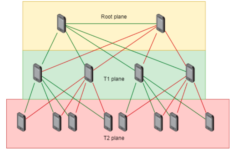
The advantage of this topology is that it does not require a complex N² discovery method. If your node and the destination node exist, a routable path is guaranteed.

2.4.2. Network Initialization¶

The network is established by a single root node. The next device to connect becomes the replicant node on the root plane. The replicant node is identical for routing but forwards all data manifest updates to the root node to ensure a single source of truth.

After the root plane is filled, child nodes can connect to parent nodes. Each child connects to two parent nodes (one primary, one secondary) to achieve redundancy. If one parent node fails, an alternate route still exists.

2.4.3. Handling Disconnects
¶

Graceful Disconnects: A node intending to leave sends a disconnect message. This signals that its published data is no longer relevant and can be deleted from the data manifest.
Ungraceful Disconnects: If a node goes out of range or its application is terminated, it is considered active until a keep-alive TTL expires. After expiration, the node is deemed dead and a disconnect procedure is initiated.

2.4.4. Connection Boundaries¶

To prevent constant, costly network hopping, connection boundaries are defined using RSSI values. A node only seeks a new connection when its current one degrades past a certain threshold. The protocol describes 6 boundaries:
- Minimum connection strength.
- Minimum connection establishment strength.
- Minimum/Maximum primary connection promotion strength.
- Minimum/Maximum secondary connection promotion strength.

Implementation-Specific Values

The specific RSSI values for these boundaries are left to the implementer, as they depend on the area of operation, device chipsets, and communication technology used.

2.4.5. Distribution Node Promotion Rules¶

When a distribution node reaches half its maximum client capacity, it triggers a promotion process. It requests a "fitness score" from all connected clients. The two nodes with the highest scores are chosen for promotion. The fitness score is calculated as follows:

flowchart TD
    %% Start Node
    Start(Start: Calculate Fitness Score)

    %% Go/No-Go Checks
    A{Has Tech<br>Capabilities?}
    B{Has > 25%<br>Battery Life?}
    C{Primary RSSI > Min<br>Promotion Strength?}
    D{Secondary RSSI > Min<br>Promotion Strength?}

    %% Calculation Steps
    E["1. Calculate Primary Score<br>Base = 100 + Primary RSSI<br>Apply penalty if RSSI > Max"]
    F["2. Calculate Secondary Score<br>Add (100 + Secondary RSSI)<br>Apply penalty if RSSI > Max"]

    %% Final Adjustment
    G{Has > 50%<br>Battery Life?}
    H["3. Adjust for High Battery<br>Subtract 10 from score"]

    %% End Nodes
    EndZero(Return Fitness Score: 0)
    EndFinal(Return Final Fitness Score)

    %% Define Flow
    Start --> A
    A -- No --> EndZero
    A -- Yes --> B
    B -- No --> EndZero
    B -- Yes --> C
    C -- No --> EndZero
    C -- Yes --> D
    D -- No --> EndZero
    D -- Yes --> E

    E --> F
    F --> G

    G -- No --> H
    H --> EndFinal
    G -- Yes --> EndFinal

Note on RSSI

RSSI values are negative, so a "higher" value is one that is closer to 0 (e.g., -55 dBm is a stronger signal than -75 dBm).

2.5. Nodes¶

This chapter describes the behavior and functionality of the different node types.

Base Functionality

Every node has the functionality of a Client Node. Distribution and Root nodes are specialized types that provide additional functionality.

2.5.1. Distribution Nodes¶

Distribution nodes form the network backbone, responsible for routing and caching data. When created, the first distribution node becomes the root node. Once five nodes are connected, the two "fittest" are promoted to become new distribution nodes, setting up their own Access Points for new clients. If a distribution node is full, it stops broadcasting its SSID until a slot becomes free.

2.5.2. Client Nodes¶

A client node is always connected to a distribution node's AP. It can publish and request data but cannot directly communicate with nodes it is not connected to. Upon connecting, it performs a handshake with the distribution node to confirm the connection and verify the integrity of the Data Manifest via a hash check. If a client loses connection, it will try to reconnect for 5 seconds before erasing its state and starting a new connection procedure.

2.5.3. Root Node¶

The root node is at the top of the network graph. It is responsible for providing the single source of truth for the Data Manifest. All updates to the manifest are sent to the root node. The root node initializes the network by creating the data structures and setting up the first Access Point with a specific SSID pattern: [mesh identifier]-[mesh name]-[Tx]-[xxxx]. This pattern is crucial for other nodes to discover the network.

2.5.4. Root Replication Node¶

This node is part of the root plane and shares routing responsibilities. However, it does not manage the Data Manifest itself unless the root node goes offline, at which point it becomes the acting root node until a new one is elected.

2.5.5. Node Connection Procedure¶

A node wishing to join first scans for Wi-Fi networks matching the predefined SSID pattern. If multiple distribution nodes are available, it selects the best one based on these rules:
1. Filter for all nodes with an RSSI above the minimum connection establishment strength.
2. From that list, select the nodes with the lowest network plane number (e.g., prefer T1 over T2).
3. From the remaining list, pick the node with the highest RSSI value (strongest signal).

This logic ensures the network grows compactly from the root outwards.

sequenceDiagram
    participant C as Client (Wi-Fi Library)
    participant CL as Client (Connection Logic)
    participant MH as Client (Message Handler)
    participant DMH as Dist. Node (Message Handler)
    participant DCL as Dist. Node (Connection Logic)

    C->>CL: Scan for all available networks
    note over CL: 1. Compare list with SSID pattern
    note over CL: 2. Filter by min. RSSI strength
    note over CL: 3. Filter by lowest plane number
    note over CL: 4. Select network with highest RSSI
    CL-->>C: Return best SSID

    C->>CL: Configure STA interface with returned SSID
    C->>CL: Connect to the network

    CL->>MH: send hello message
    MH->>DMH: hello message
    DMH->>DCL: source IP address
    DCL-->>DCL: Add IP to TTL table

    DMH-->>MH: Return hello ack message
    MH-->>CL: Receive hello ack message
    CL-->>CL: Add IP to TTL table

Figure: The swimlane diagram illustrating the node connection process.

2.5.6. Node Hopping and Connection Recovery¶

If a client node's connection degrades past a boundary, it sends a disconnect message and searches for a new parent. If a distribution node's connection degrades, it first tries to promote one of its own clients to take its place. If no clients are fit for promotion, it sends a disconnect message to its children and gracefully leaves the network.

2.5.7. TTL and Keep-Alives¶

Keep-alive timers ensure connectivity on unreliable connections. Each connection has a timer, and keep-alive messages are broadcast periodically to reset them. The TTL value is a critical tuning parameter: - Short TTL: Better for highly dynamic networks with frequent disconnects, but increases traffic.
- Long TTL: Better for more static networks, as it reduces data traffic.

2.6. Defining the Routing Method¶

2.6.1. Network Routing¶

The routing over this network happens according to the following rules. First, the node checks if the destination address is its own address. If so, the message is passed to the message handler.

If the destination is not the local address, a check is performed to see if the address is a valid network address. If it is, the routing logic proceeds based on the interface the message arrived on:

If a message arrives from the STA interface (from a parent/up the tree):
- The message is forwarded to the destination if it is reachable on one of the node's child branches.
- The message is dropped if the destination is not reachable through this node's child branches.
If a message arrives from the AP interface (from a child/down the tree):
- The node checks if the destination is reachable on another child branch. If so, it forwards the message to that branch.
- Otherwise, the message is sent up the tree to the parent node.

flowchart TD
    A(Packet Arrives at Node) --> B{Is Destination == Local IP?}
    B -- Yes --> C(Pass to Message Handler)
    B -- No --> D{Which Interface Received Packet?}

    D -- STA (from Parent) --> E{Is Dest in any Child Branch?}
    E -- Yes --> F(Forward to Child Branch)
    E -- No --> G(Drop Packet)

    D -- AP (from Child) --> H{Is Dest in another Child Branch?}
    H -- Yes --> I(Forward to other Child Branch)
    H -- No --> J(Forward to Parent)

To know if a destination node is reachable on the current branch, the following calculation is performed.

// --- Define Input Variables ---
Pl = local_ip.third_octet
Ll = local_ip.fourth_octet
Pd = destination_ip.third_octet
Ld = destination_ip.fourth_octet

// --- Calculate Distances ---
Plane_distance = Pd - Pl

// --- Determine Reachable Bounds based on Node Position ---
if (Ll % 2 == 0) {
    // Logic for EVEN numbered nodes
    Reachable_upper_bound = Ll * (2^Pd)
    Reachable_lower_bound = Reachable_upper_bound - (4 * Plane_distance)
} else {
    // Logic for ODD numbered nodes
    Reachable_upper_bound = (Ll + 1) * (2^Pd)
    Reachable_lower_bound = Reachable_upper_bound - (4 * Plane_distance)
}

// --- Final Check ---
if (Ld >= Reachable_lower_bound AND Ld <= Reachable_upper_bound) {
    return REACHABLE
} else {
    return NOT_REACHABLE
}

If the local node's position (Ll) is an even number:

A destination is considered "on the current branch" if its position (Ld) is within the calculated Reachable lower bound and Reachable upper bound.

Interface Selection

Each node has two station interfaces. A message will always be sent through the interface whose address has a fourth octet that is mathematically closest to the fourth octet of the destination address.

2.6.2. Network Address Translation (NAT)¶

NAT is used between distribution and client nodes. Since the protocol listens on a specific port, a NAT ID field is added to the protocol header to identify the source client when forwarding messages into the distribution network and back.

2.6.3. Message Handler¶

The message handler sorts incoming packets by message type and calls the appropriate logic function, acting as the central traffic controller for the node.

2.7. Data Definition¶

2.7.1. Packet Format¶

The protocol uses a custom header inside the data field of a standard UDP packet.

|         8bit        |        8bit         |        8bit        |        8bit        |
---------------------------------------------------------------------------------------
|                                32-bit Source Address                                |
---------------------------------------------------------------------------------------
|                              32-bit Destination Address                             |
---------------------------------------------------------------------------------------
|  Message Type (8)   |       TTL (8)       |      NAT ID (8)    |     Reserved (8)   |
---------------------------------------------------------------------------------------
|                                                                                     |
|                                                                                     |
|                                20 bytes (160 bits)                                  |
|                                      SHA1 Hash                                      |
|                                                                                     |
|                                                                                     |
---------------------------------------------------------------------------------------
|                                                                                     |
.                                                                                     .
.                                MAX 65,448 bytes of Data                             .
.                                                                                     .
|                                                                                     |
---------------------------------------------------------------------------------------

Header Part	Size (bits)	Description
Source Address	32	`192.168.x.x` of the originating node.
Destination Address	32	`192.168.x.x` of the target node.
Message Type	8	Defines packet purpose (see table below).
TTL	8	Time To Live.
NAT ID	8	Identifier for NAT translation.
Reserved	8	For future use.
SHA1 Hash	160	Hash of the data payload for integrity checks.
Data	up to 65,448 bytes	The actual message payload.

Segmentation

The current protocol does not handle packet segmentation. For messages larger than the maximum data size, a custom implementation would be required to split the data and re-assemble it, ensuring the custom header is stripped before processing.

2.7.2. Message Types¶

The message type field in the header dictates how the packet is handled.

Message Type	Value	Cacheable
default message	0	no
Hello message	1	no
Promotion message	2	no
Promotion ack message	3	no
Keep alive message	4	no
data manifest request	5	no
data manifest ack	6
cacheable data message	7	yes
data manifest broadcast	8	no
data manifest delta broadcast	9	no
Promotion fitness request	10	no
Promotion fitness response	11	no
publication request	12	no
publication request response	13	no
Disconnect message	14	no
User defined	20-30	yes
User defined	30-40	no

Reserved & User-Defined Types

Values 7-19 are reserved for future system messages. Values 20-40 are available for custom, user-defined message types, provided a callback function is supplied to the message handler.

2.7.3. Data Manifest Table The Data Manifest is a table present on each node that holds the UUID and location (IP address) of published data. This could be anything from a website URL to the ID of a smartphone for direct messaging.

Example Data Manifest

Unique Identifier	IP Address
record 0	192.168.0.2
record 1	192.168.3.4
record 2	192.168.9.10

To handle routing to specific client nodes, each distribution node also maintains a Local Manifest Table, which maps the data's UUID to the client's NAT ID.

Example Local Manifest Table

Unique Identifier	NAT ID
record 0	2
record 1	4
record 2	3

The Data Manifest is versioned with a 32-bit integer. All modification requests are sent to the root node, which updates the master table and broadcasts the new version to the network. If a node disconnects, the distribution node it was connected to is responsible for removing its data records from the manifest.

2.7.4. Data Caching To minimize network traffic, distribution nodes can cache data from packets marked as cacheable. When a request for cached data is received, the node first sends the data's hash to the original source. The source verifies if the data is still valid.

If valid, the source sends an ack message, and the distribution node serves the data from its cache. If invalid (e.g., the data has been updated), the source sends the new data, which the distribution node then caches and forwards.

Example Data Cache Table

Unique Identifier	Hash	Manifest Location	Data Location Pointer
record 0	SHA1 Hash	Record 1	0xFFFF
record 1	SHA1 Hash	Record 0	0XFFFF
record 2	SHA1 Hash	Record 3	0xFFFF

2.8. Implementation Considerations¶

2.8.1. Security Considerations¶

Zero-Trust Network

This network should be considered insecure by default. While individual links are secured with WPA3, the network password is known by all nodes. It is essential that any application built on this network uses a zero-trust model and implements its own end-to-end encryption for any data that needs to remain private.

For secure networks, it is advised to have the host generate a random password and distribute it via a secure out-of-band method, such as scanning a QR code.

2.8.2. SSID Patterns and Provisioning¶

The SSID pattern [mesh identifier]-[mesh name]-[Tx]-[xxxx] is critical for network discovery. This pattern can either be hard-coded during implementation or supplied at runtime (e.g., via a QR code) to allow for multiple, distinct mesh networks.

The protocol is designed for Wi-Fi 6 and uses a single symmetric key (password) for the entire network. This key can be a predefined "provisioning key" for public networks or a unique password set by the host for private networks. To prevent unauthorized access, these keys should be stored securely on the device, for example, in a hardware-backed password vault.

2.9. Bibliography¶

[1] J. Postel, „User Datagram Protocol,” RFC, 28 August 1980.
[2] J. Moy, "OSPF Version 2," RFC 2328, April 1998. [Online]. Available: https://www.ietf.org/rfc/rfc2328.txt.

Of course. I will format those sections into clean, readable Markdown tables as requested.

Here is the formatted output:

3. Submissions: The Research & Validation Roadmap¶

To validate and evolve this protocol, we will complete the following major submissions.

Objective ID	Submission Title	Core Goal	Status
`5_1_6_6...`	Peer Review of Protocol v0.1	To submit this document to external network scientists for peer review and feedback on its soundness.	Planned
`5_2_6_6...`	Simulation and Modeling	To create a network simulation to test the protocol's behavior under various stress conditions (e.g., mass disconnects).	Planned
`5_3_6_6...`	Performance Benchmark Definition	To define the Key Performance Indicators (KPIs) that the real-world implementation must meet to be considered a success.	Planned

4. Role Management: Call for Contributions¶

This is a deep research project, and we need brilliant minds to ensure its scientific rigor.

Role ID	Role Title	Your Mission If You Join
`4_3_6`	Mesh Network Researcher	You will analyze, challenge, and improve the core routing and promotion algorithms defined in this protocol.
`4_8_6`	Computer Scientist (Simulation)	You will build the software models that simulate the Onlife network at scale to find its breaking points before we write a line of app code.
`4_9_6`	Security Analyst	You will analyze the protocol for theoretical vulnerabilities and help design a robust security model for applications built on top of it.

5. Team Budget¶

Item	Value (SC)	Status
Total Phase 1 Budget:	0	Awaiting initial crowdfunding
SC Minted to Date:	0	-
Remaining Budget:	0	Our first goal is to meet the Validation Phase crowdfunding target.